|
|
Abstract
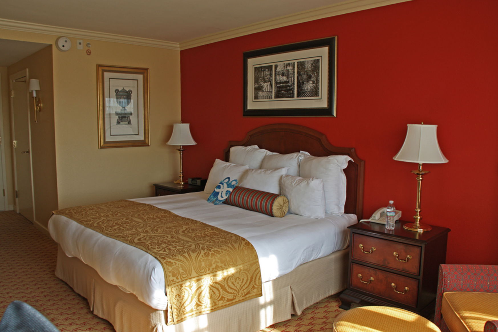
In this project, our goal was to take in a 2D image as the only input, and be able to render an artificial object into the scene with realistic lighting and shading. We were inspired by this [1] paper by Kevin Karsch et al., and sought to reproduce its results. In order to do this, we had to put together a number of steps: finding a depth map and reconstructing a mesh of the original scene, finding the true colors of objects in the scene, estimating the direction and intensity of lighting, and finally rendering in objects in a way that looks clean and close to the original image. Along the way, we had to constrain the problem to assume all objects in the scene with diffuse, that only indoor scenes would be reconstructed, and that reflective objects would not be rendered in. Using a number of libraries in addition to the NVIDIA OptiX raytracer framework, we were able to generate convincing images.
Technical Approach
Scene Reconstruction
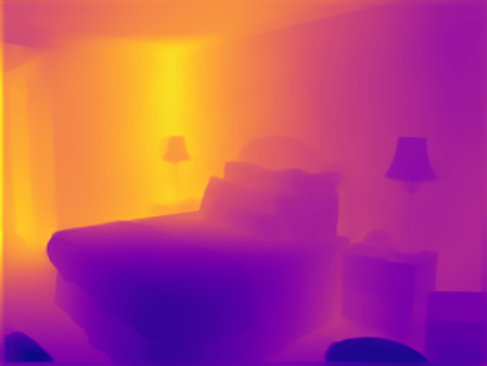
Depth Estimation
To reconstruct the scene, we used a number of existing libraries and frameworks, as it was not the focus of our project. For depth estimation in the scene we resize the image to 320x240 and used this [2] program by Ibraheem Alhashim and Peter Wonka, whcih uses transfer learning on an NYU dataset of indoor scenes in order to estimate a depth map based on the image. We explored a wealth of literature and tested a number of different libraries on this topic, such as the method used by the original Karsch paper, and methods that directly estimated the resulting mesh by finding planar surfaces, but found by far the best results with this library.
|
|
|
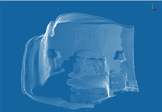
Point Cloud Operations and Mesh Reconstruction
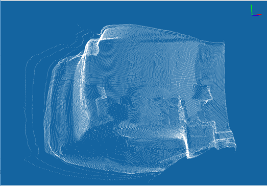
From the depth map, we assume that the image was taken with a pinhole camera and assume an arbitrary field of view, and use spherical coordinates to create a create a point cloud. We generate a .pcd file format so we can use the Point Cloud Library (PCL) [3] to filter the cloud and generate the mesh. We first filtered the mesh to remove outlier points, so that distinct surfaces at different depths would not be erroneously connected to one another, making occlusion possible. The algorithm was fairly simple; considering a group of 50 nearby points, remove any points more than 2 standard deviations away from the mean. This filtering was done by the PCL.
|
|
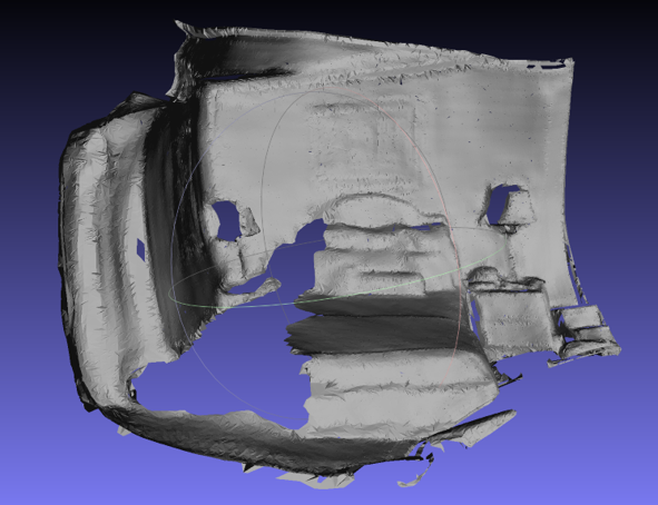
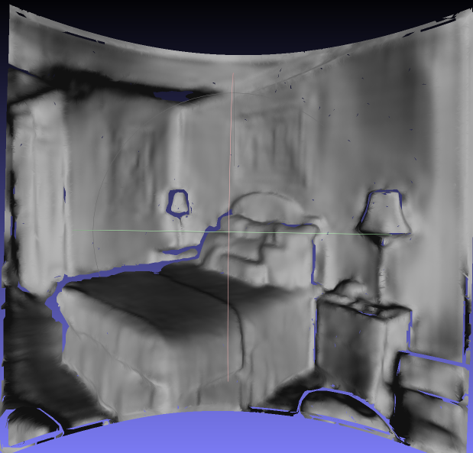
Then, we use the PCL's Greedy Projection Triangulation to quickly reconstruct a mesh. We researched alternatives, but as this wasn't the focus of the project, we decided to use a library to get a fast, clean mesh.
|
|
Note the gaps behind the bed out of view of the camera, a result of point cloud filtering. This enables occlusion of objects rendered in.
True Color Estimation
To estimate the true color of objects in the scene in the absence of lighting, we use the PDE-retinex algorithm as described in this [4]
paper by Nicolas Limare et al. This must be done because we don't want our shading effects to be computed on the already lit/shadowed colors of objects in the scene; we want our shadows to be computed with respect to the scene's "intrinsic color".
The algorithm aims to get rid of shading effects by assuming that changes in color due to shading will be smooth, while the boundaries between patches will be relatively sharp. It thus
strives to preserve sharp boundaries between color patches while evening out the interiors of those color patches.
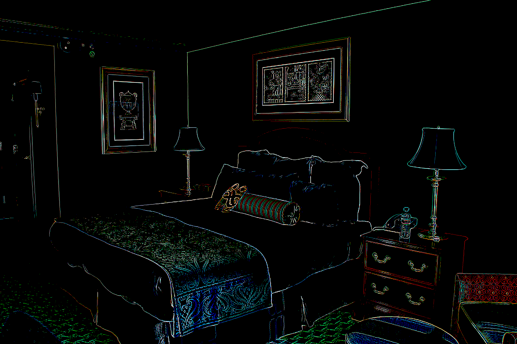
The algorithm operates independently on each color channel, and begins by applying the Discrete Laplacian Transform:
$F(i, j) = f(I(i, j) - I(i-1, j)) + f(I(i, j) - I(i, j-1)) + f(I(i, j) - I(i+1, j)) + f(I(i, j) - I(i, j+1))$
where I(i, j)
is the pixel value at that point in a certain color channel, and f() is a threshholding function that only keeps a value if it is larger than a predetermined
threshhold. This essentially operates as an edge detector: edges of sharp color gradient in the image are emphasized.
|
The Discrete Fourier Transform of F is then computed, and the following function is applied with m and n as height and width. This transform solves a Poisson equation, which has the effect of preserving gradients present after the DLT, and setting all other gradients to 0.
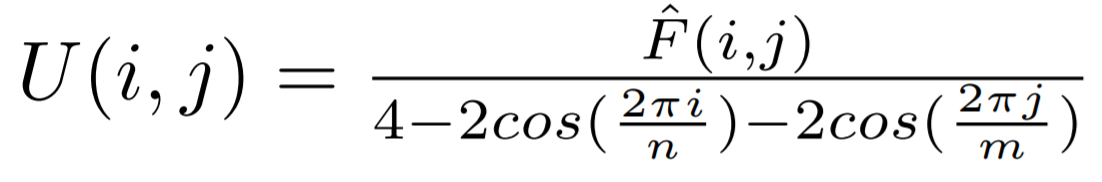
|
The inverse DFT is applied, and the result is normalized to share the same mean and variance as the original image.
|
|
|
Lighting Estimation
For lighting estimation, we aim to determine the position of the lights in the scene in order to accurately shade the model. To make the problem easier, we assumed that the lighting of the scene was sufficiently far away from the scene that the lighting model can be approximated with an environment map. We see here that the problem essentially reduces to image to image translation.
We used the Laval indoor HDR panorama dataset [7] for illumination estimation. That dataset has a very rich dynamic range, using 32 bit floating point numbers to represent each channel. The images manage to capture the full range of illumination without having the lights washed out. This is very important to our problem because this means that the illumination from the light sources are proportional to how they are in real life. We used Tensorflow 2.0 to create a convolutional neural network that takes in 64x64 images and returns a 64x64 light map of the scene. We prepared the dataset by cutting out squares from the middle of each panorama corresponding to the approximate field of view of a cell phone camera. We then brightened the image and upper bounded it in order to get that image to resemble a photogaph taken by an ordinary camera. We then feed this image into the neural network and try to get it to predict the full size panorama.
|
|
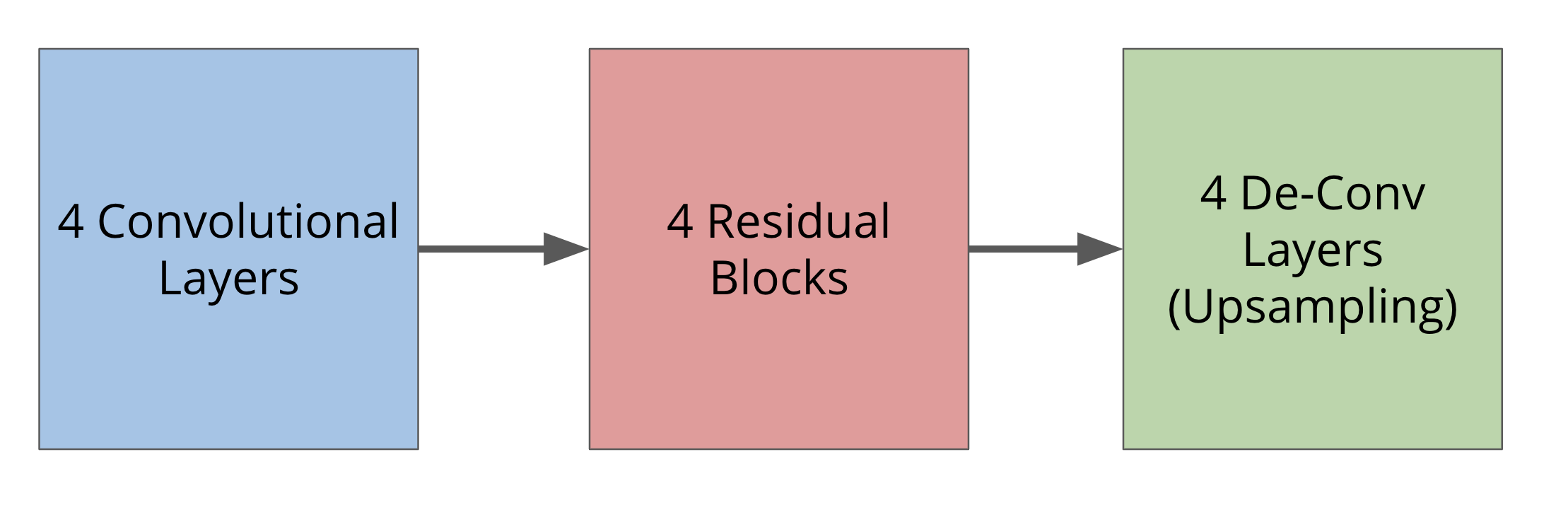
A high level overview of the model is shown below. Each Conv2D Layer has 4x4 kernels, stride 2, and “Same” padding. The first layer has 32 filters, and doubles by two every layer. Each Residual Block has 3 convolutional layers, each followed by a Batch Norm and a leaky ReLu activation. Then, the input of the block is appended to the output. Each upsample layer consists of first upsampling the image (to reduce checkerboarding artifacts), then a convolutional layer with stride 1, then instance-norm and leaky-relu. The last layer is followed by a tanh activation.
|
A key difference between this problem and most other image to image translation problems is that the desired information is low frequency. Furthermore, we care more about the distribution of the light as a probability function. This is because we are mainly using diffuse scenes, where the brightest parts of the image matter the most. Taking this into account, we used cross-entropy loss instead of L1 or L2 loss which is normally used for this purpose. Cross entropy loss essentially minimizes the K-L divergence between the target image and the predicted image. This means that the model will train better and learn the brightest parts of the image.
Given limited time and computational power, we unfortunately did not have enough time to train a fully functional model. The model underfit, but did learn that most of the light from the image comes from the back of the image. While this works for most images, we tried to switch to a more direct method of calculating illuminance.
To remedy this issue, we turned to a method inspired by Marschner [8]. The key insight is that rendering is linear with respect to the environment map we're using. So, we can combine lightings by just taking the linear combinations of the output images from rendering with the individual lights. In order to find an approximate light map, we render 16 images with the predicted mesh from above, each with an environment map corresponding to a different portion of the scene being illuminated. We turn these into column vectors, \( \vec{v_1}, ..., \vec{v}_{16} \) and combine these into one matrix, \(\mathbf{V}\). Then, if \(b\) is our original image, we use least squares to solve the system \(\mathbf{V}\vec{x} = \vec{b} \). x in this case corresponds to the coefficients of the original environment maps. We then take the linear combination to get the final light map. Unlike Marschner, we used a equirectangular system to parameterize the environment map to simplify the implementation, finding this sufficient for the types of indoor scenes that we were dealing with.
However, we found that many of the relit basis images are very close to being linear combinations of each other, especially if the light ends up behind the scene. This means that the matrix has very low singular values, causing numerical instability and coefficients with very negative values. We regularize by using another idea in the paper: reduce large changes in adjacent lighting cells in the basis lighting maps. We can do this by creating another matrix \(\mathbf{B}\), which has a row for every two neighboring cells. Each row has a 1 in the column of the first cell, and a -1 in the column of the other. Then, multiplying this by \(\vec{x}\), we get another vector, which we want to minimize to zero. We can do this at the same time as doing the above least sqaures problem by appending \(\mathbf{B}\) below \(\mathbf{V}\) and zeroes below \(\vec{b}\): \[ \begin{bmatrix} \mathbf{V} \\ \lambda\mathbf{ B} \end{bmatrix} \vec{x} = \begin{bmatrix} \vec{b} \\ \vec{0} \end{bmatrix} \] Here, \(\lambda \) is a parameter to adjust regularization.
|
|
One lesson we learned when working on lighting estimation was that the simplest techniques often trump those that are in vogue. Initially, we were excited to use deep learning to automatically predict lighting because of the impressive results obtained by Gardner and others. Our final CNN model was satisfactory at best, though given more compute time, we may have been able to optimize the model further. The least-squares approach employed by Marschner was sufficient for our purposes, which was a pleasant surprise considering that it was published nearly two decades ago. All in all, it was instructive to explore both modern and classical techniques for the lighting estimation problem.
Rendering
Because the lighting estimation stage was so render-intensive, we re-implemented Project 3 (Pathtracer) using NVIDIA OptiX [5], a framework that enables ray tracing on the GPU. With OptiX, one writes CUDA C code to define ray tracing operations for individual pixels that are easily parallelized across the image. Since much of the Project 3 code for importing meshes and environment maps was handled by the staff-provided starter code, we had to implement these features from scratch to be compatible with OptiX. Moreover, NVIDIA recommends that path tracing be implemented iteratively rather than recursively, so it took special care to account for the various multiplicative factors involved in global illumination. Needless to say, it took many days of debugging before our OptiX version of Pathtracer matched that of Project 3. We also spent a long time getting the scene to align just right with the raytracer so that the render would be at exactly the same vantage point as the original image.
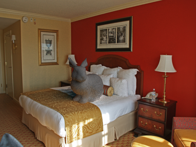
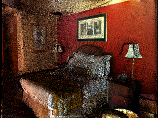
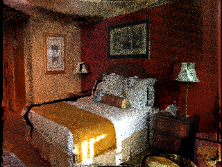
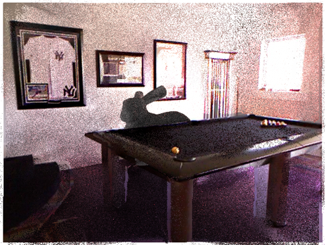
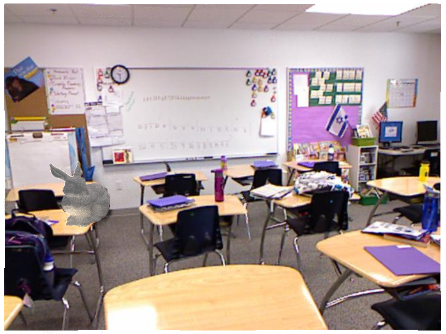
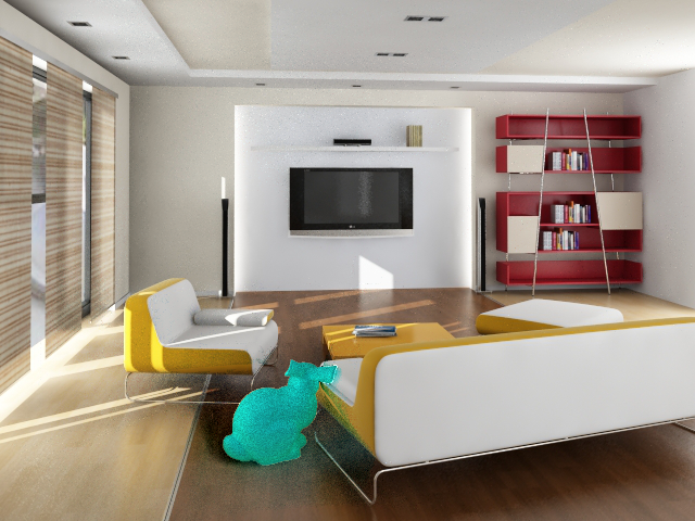
Our first approach at the actual render was as follows: for each pixel, check whether the rays at that pixel would eventually intersect the object being rendered in. If they did not, simply use the pixel value from the original image and ignore the scene altogether. If they did intersect the object, use the lighting estimation and retinex output to compute the output pixel value. Some results of this algorithm are shown below:
|
|
This was not a complete failure; shading effects are cleary visible, and where they would be expected to be. In addition, occlusion behind objects in the scene is possible, as a result of the cloud filtering done during scene reconstruction. The extreme noise is because checking whether a certain pixel's rays intersect the object introduces randomness in whether neighboring pixels are chosen to be fully computed or default to the original pixel value. This is why areas of the scene that are out of line-of-sight of the bunny are entirely free of noise; they simply use the original image.
Differential Rendering
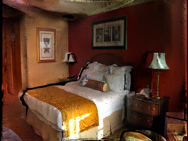
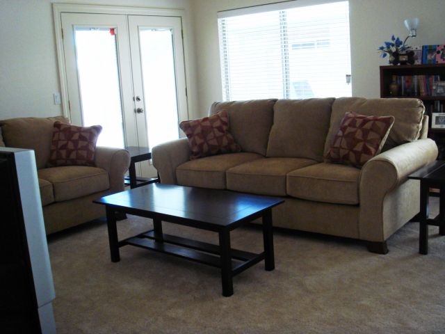
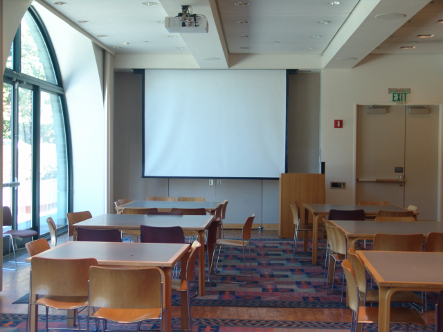
Inspired by the approach taken by Karsch [1] and by this paper [6] by Paul Debevec, we fixed the aforementioned noise issue using differential rendering. First, we rendered the scene without the added object, using the retinex output.
|
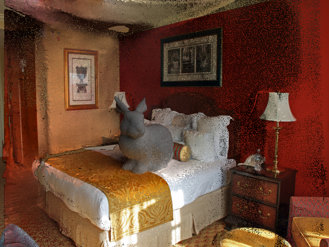
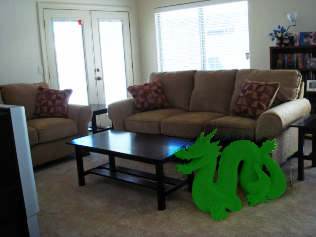
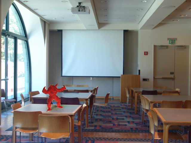
Then, we subtract this rendered image from the original image to compute an "error term". Render the object in as before, except for each pixel whose rays we determined as interacting with the object, we now add in the precomputed error term.
|
|
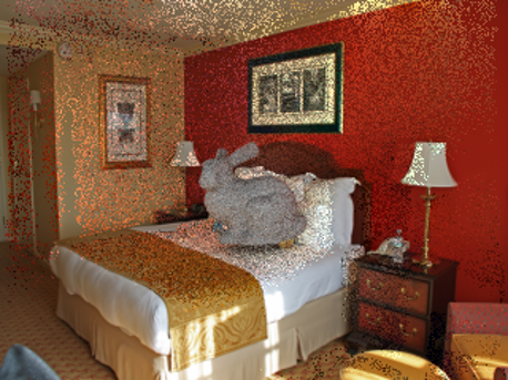
The result is a much less noisy image, as differences between the new render, which uses our lighting estimation and retinex values, and the original image are mostly accounted for by this error term.
We slightly modified Debevec's method by only adding the error term to pixels that actually "interacted" with the synthetic object: that is, pixels for which at least one path of light hit the object. This effectively reduced render times by a constant factor because we were able to shoot a number of "test rays" through each pixel to check if they ever bounced off the object, and then decide to use the global illumination estimate (plus the error term) or the original image's pixel value accordingly. We decided to implement this modification because it seemed appropriate that render time scale with the proportion of the scene with which the object interacts.
The main lesson we learned from re-implementing path tracing was the importance of integration testing, visual debugging, and a full understanding of the mathematics behind radiance calculations. It often was the case that we implemented a feature such as cosine-weighted hemisphere sampling and tested it for correctness using direct lighting with the bunny model alone only to discover a couple days later that global illumination produced images that were too bright due to an incorrect probability density calculation. Tracing the source of such issues was painful, but we became well-versed in visual debugging as a result. To deal with other issues involving numerical precision for the marginal probability distributions used in environment mapping, we had to think about how to make these calculations robust with 32-bit precision (since OptiX only permits floats to be passed to the GPU). Overall, we gained an appreciation for much of the skeleton code in Project 3 as we had to implement this functionality more or less from scratch to interoperate with OptiX.
Results
|
|
|
|
|
|
|
|
Final Video
References:
- "Automatic Scene Inference for 3D Object Compositing", Kevin Karsch et al., 2009 http://www.eecs.harvard.edu/~kalyans/research/auto3d/AutoSceneInference_TOG14.pdf
- "High Quality Monocular Depth Estimation via Transfer Learning", Ibraheem Alhashim and Peter Wonka, 2018
https://arxiv.org/abs/1812.11941
- Used the accompanying implementation at https://github.com/ialhashim/DenseDepth
- Point Cloud Library http://pointclouds.org/
- "Retinex Poisson Equation: a Model for Color Perception", Nicolas Limare et al., 2011 http://www.ipol.im/pub/art/2011/lmps_rpe/
- NVIDIA OptiX https://raytracing-docs.nvidia.com/optix/guide/index.html#guide#
- "Rendering Synthetic Objects into Real Scenes: Bridging Traditional and Image-Based Graphics with Global Illumination and High Dynamic Range Photography", Paul E. Debevec, 1998 https://www.pauldebevec.com/Research/IBL/
- "Learning to Predict Indoor Illumination from a Single Image", Marc-André Gardner et al., 2018 http://vision.gel.ulaval.ca/~jflalonde/projects/deepIndoorLight/
- "Inverse Rendering for Computer Graphics", Stephen R. Marschner, 1998 http://www.cs.cornell.edu/~srm/thesis/
Contributions
- Anup Hiremath: Focused on depth estimation, point cloud filtering, and mesh reconstruction. Also implemented PDE-retinex.
- Gaurav Rao Focused on lighting estimation.
- Jay Shenoy: Focused on rendering.
All members shared ideas, researched approaches, and helped debug all parts of the project.